How to Export Primavera P6 Data into Power BI

Project planners and schedulers spend a lot of time doing repetitive work in Excel. Its not uncommon to spend 20% of your time updating Primavera P6 and 80% of your time creating the final report in Excel.

The purpose of this tutorial is to show how the Primavera P6 report generating feature along with Power BI can allow you to quickly and accurately export complex data out of Primavera P6 and create understandable reports for other project members. I have found this feature very valuable in giving the project team a better understanding of the project plan and creating more confidence in my role as a project planner.

This tutorial is based on the following scenario: You have been asked to export the resource loading data from P6 into Excel to allow a project manager to investigate the resource usage of each work group over time. You are expecting a lot of changes to the schedule and resource curves due to the project deadlines and resource constraints. How do you export the data quickly and accurately to Excel every time you get project feedback?

Before you do this tutorial, please make sure that your version of Excel is more recent than 2014 and has a Data tab available in the ribbon at the top.

The tutorial is broken into two parts.

1. How to export the resource assignments out of Primavera P6 into a CSV file using the report generating function.
2. How to use Power Query in Excel to format the CSV file into a format that can be used in Power BI or Excel.

Part One – Exporting a CSV file from P6

The first step is to set up the report generating option within Primavera P6 to generate a CSV file that contains the budgeted and budgeted cumulative hours spread over a month interval. This data will be in the same data format that you see when you click the resource assignment screen within Primavera P6.

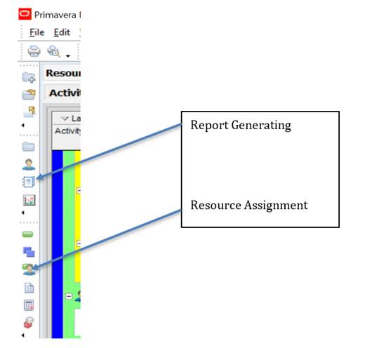
Step 1

Add a new report to the Report section of Primavera P6.

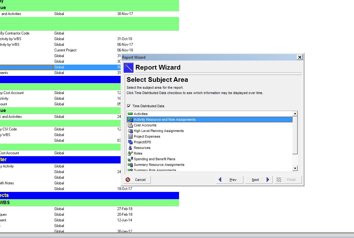
Step 2

Using the report generating wizard, make sure to click the Time Distribution Data check mark, then click the Activity Resource and Role Assignments item.

Step 3

The next screen allows you to set the Columns, Group and Sort, and Filters that you want applied to the report. For this simple report example, we will only set the Columns option. Select and add Resource Name as the only column in the report.

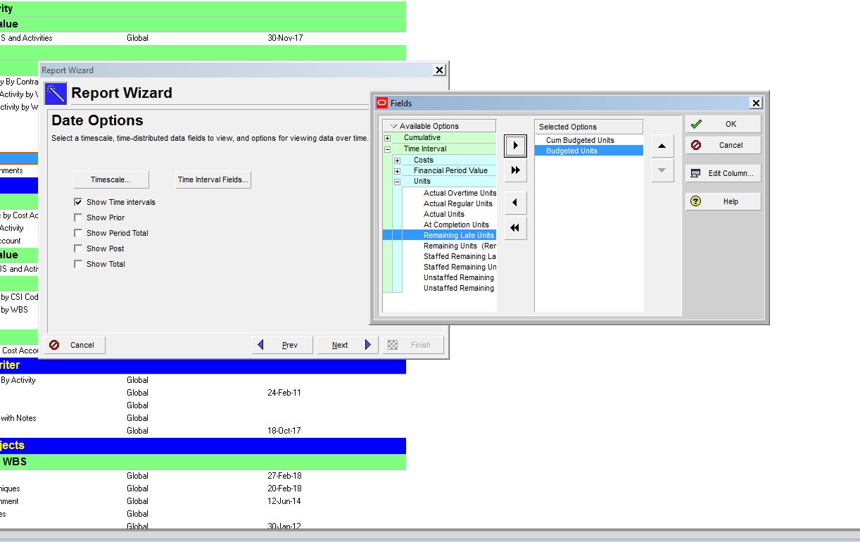
Step 4

The next screen allows you to set the data that you want to see in the time distributed report. Click on Time Interval Fields and select Cum Budgeted Units and Budgeted Units.

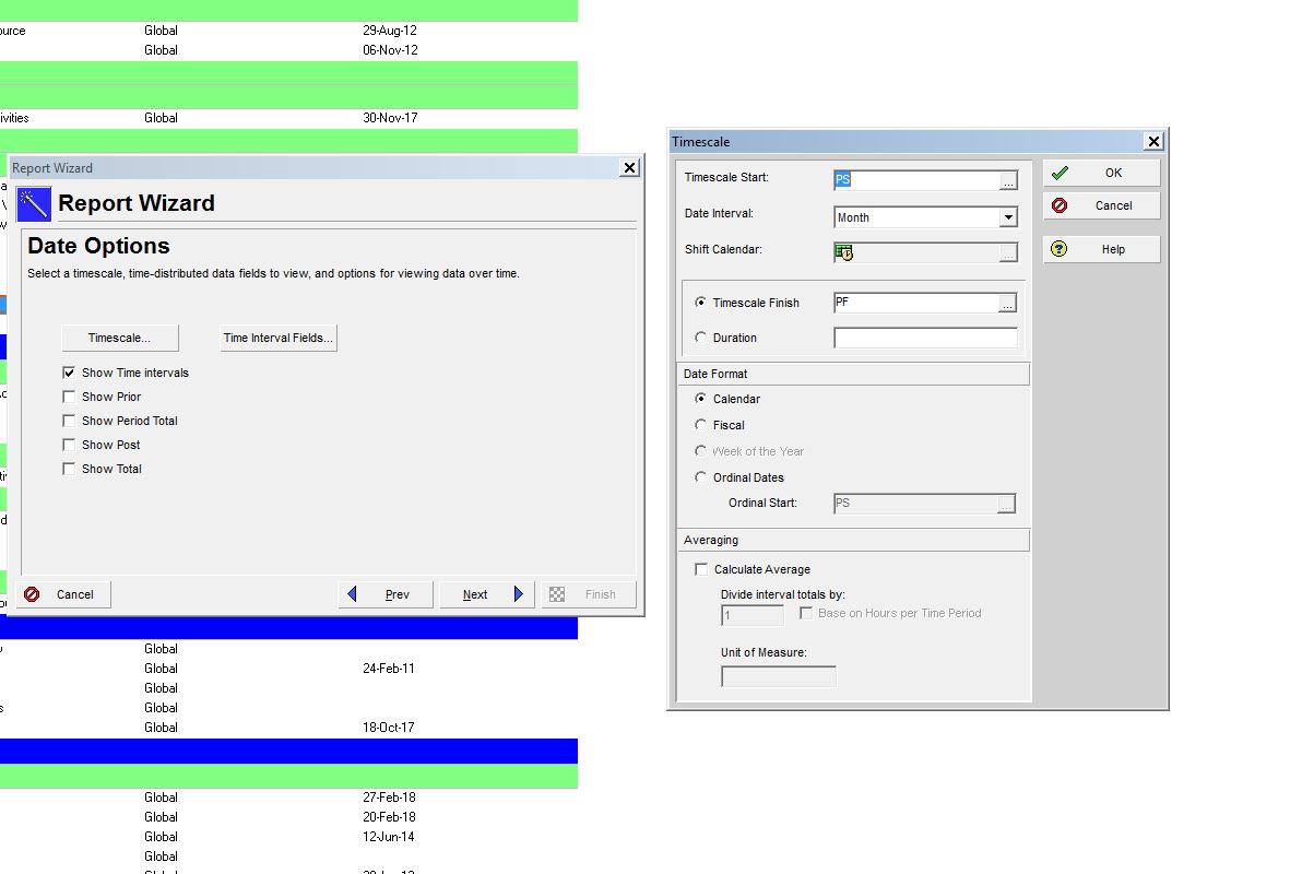
Step 5

On the Timescale option, set the Date Interval to Month.

Step 6

Click Run Report. To select the format that the report will be exported in, select the ASCII Text File option and just use the default options that P6 uses.  Set the location for the text file that P6 will export under Output file.

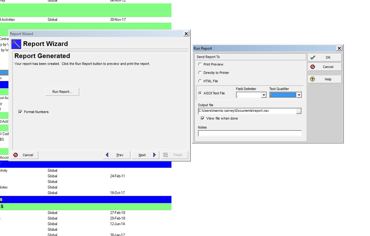
Step 7

Click Finish, and you now have a saved report that can be run against any project in Primavera P6.

 

Part Two – Importing a CSV File into Power BI Using Power Query.

 

The next step is to take the CSV file and convert it into a table format that can be analyzed using a Pivot Table or Pivot Chart. The big advantage to this technique is that in the future, when you export the CSV file again, you can simply refresh the excel workbook and the data will be updated.

Step 1

The first step is to go to the Data tab in excel and click on the Get Data option.

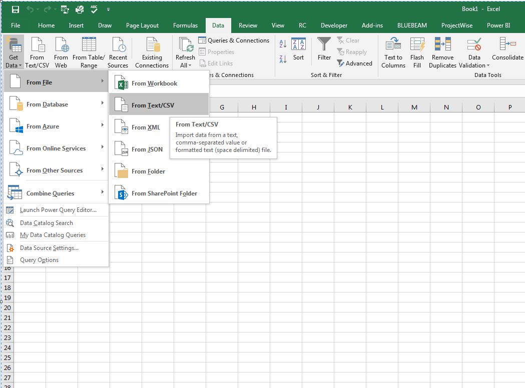
Step 2

Click From Text/CSV. You will have to go to the folder that you exported the CSV file into from P6.

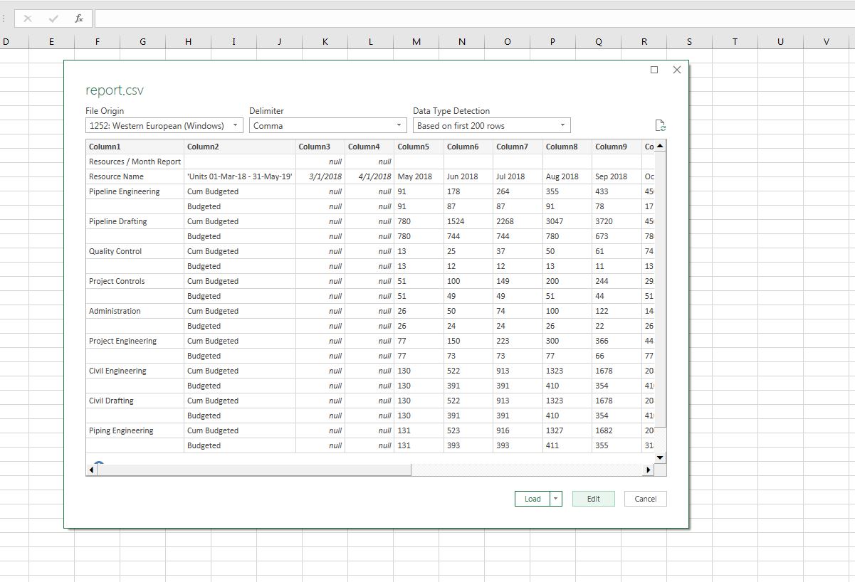
Power Query will preview the CSV file and parse it into a table format. Now open Power Query and use the interface to shape the data into a format that you can use. Click Edit in order to do this.

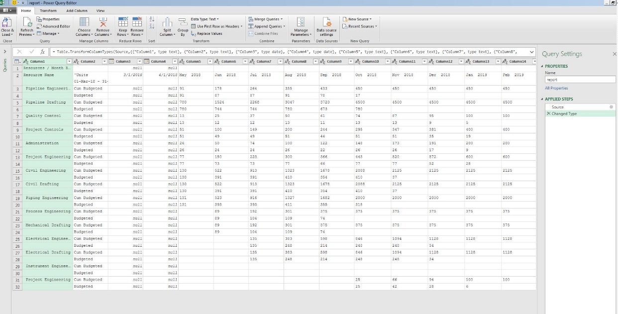
Step 3

This is the Power Query interface. The transformations that you will add are listed on the right-hand side of the screen.

The first transformation that you want to perform is in Column 1. The resource names apply to both the Cum Budgeted row and the Budgeted row. The Primavera P6 export, however, skips the second row. You need to correct this and display the resource name in both rows.

Step 4

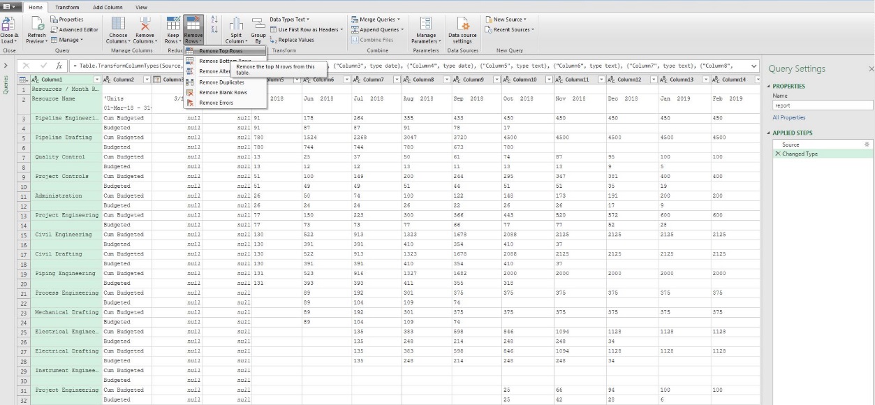
Depending on your version of Excel, Power Query may handle the data differently. You want the date row to be in the first row of the table so that you can promote them as table headers later on. If your table has the dates in row one, do nothing. If row one contains empty cells, follow the next step to remove the empty row and position the date rows in the correct place.

Click on the Remove Top Rows option, enter 1 into the pop-up box and click OK.

Step 5

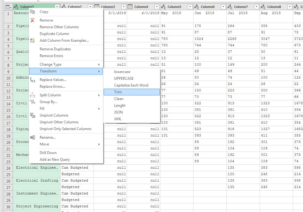
Now you need to correct the data in Column 1. First, you want to remove the spaces around the text in Column 1 by using the Trim feature. To do this, right click on Column 1, go to Transform and then click Trim.

Step 6

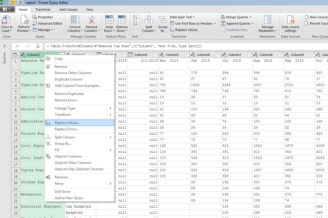
There is still a problem. You want the blank spaces in Column 1 to contain null for the next step. To do this, right click on Column 1 and select Replace Values…

Step 7

In the pop-up box, leave the Value to Find box blank as that represents the empty spaces. In the Replace With box type in null and click Ok. The spaces now contain nulls.

Step 8

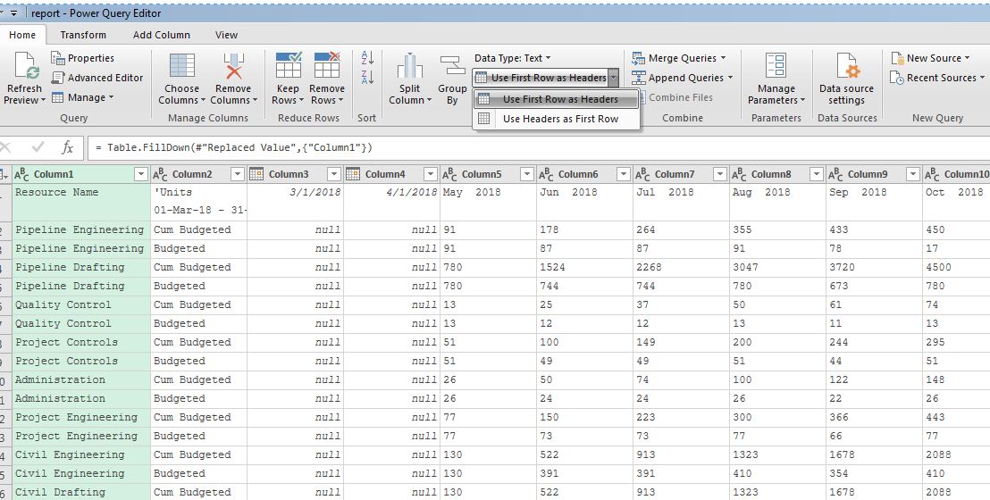
Now right click on Column 1 and select Fill and then Down. Now the Resource Names in Column 1 are correctly tagged to each row.

Step 9

The second transformation is to unpivot the time distributed data into two columns; one containing dates and one containing hours. Technically you are normalizing the data. Primavera P6 displays the data in a way that is easy for humans to read and understand. You want to undo this step and create a very long table that can be used by the Pivot Table and Pivot Chart features in Excel. Both pivoting and unpivoting data are very useful features in Power Query.

You want to use the data in Row 1 as the column headers on the table. Double check that the monthly dates for the resource distribution are in Row 1.  Then click the Use First Row as Headers option.

Step 10

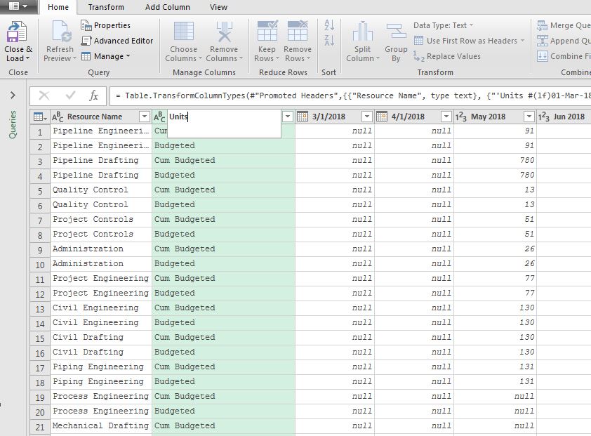
The title on Column 2 is not what you want. Rename it to Units by double clicking on t

he column header.

Step 11

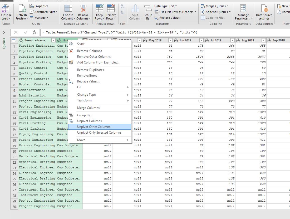
Now for the unpivot step. This is where you take the time distributed columns and rearrange that data into one single column that can be used in a pivot table. You want to unpivot the date columns only. In the future, you may extend the schedule and add more date columns. To allow the query to work in the future, you select the first two columns, right click and select Unpivot Other Columns. This unpivots all the data columns for Budgeted Units and Cumulative Units into the format that you need.

Step 12

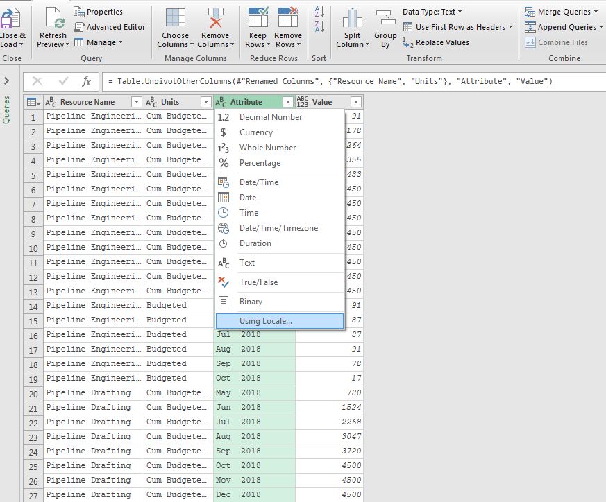
The date column is called Attribute and is categorized as text. You want to change this to a date field. You also want the date field to show correctly even if you email the file to another country where the end user has a different date format on their computer. To do this, you click on the icon to the left of the column title and click Using Locale…

Step 13

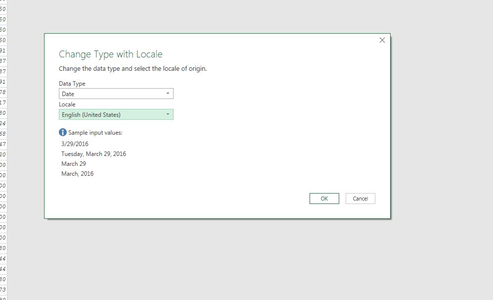
In the drop-down menu, change Data Type to Date and Locale to English (United States). You will want to use whatever Locale is setup on your computer.

Step 14

Now go to the Value column, click on the icon to the left of the column title and select Decimal Number.

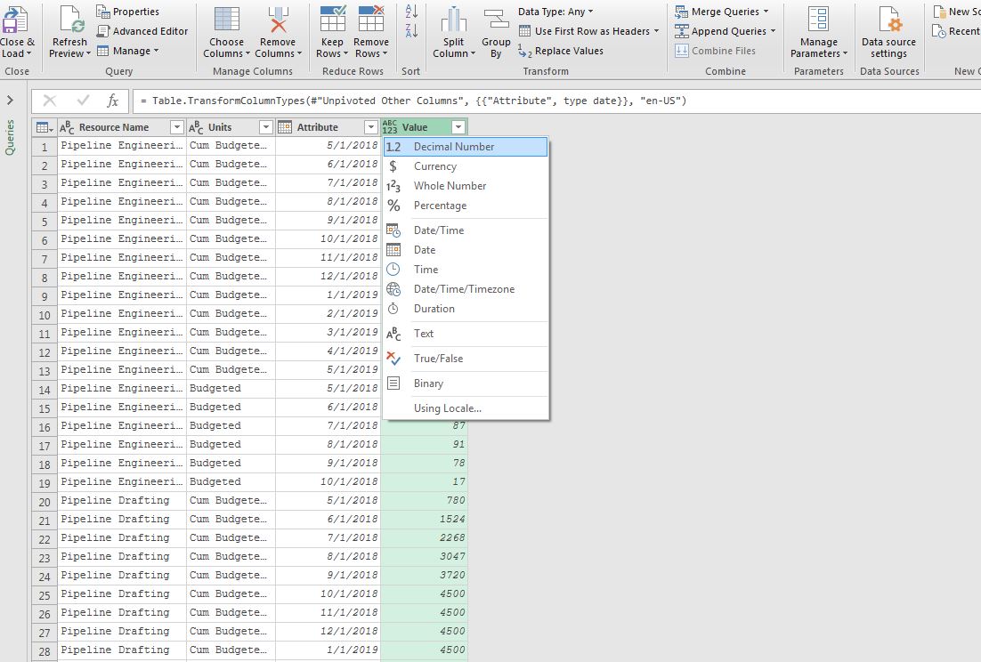
Step 15

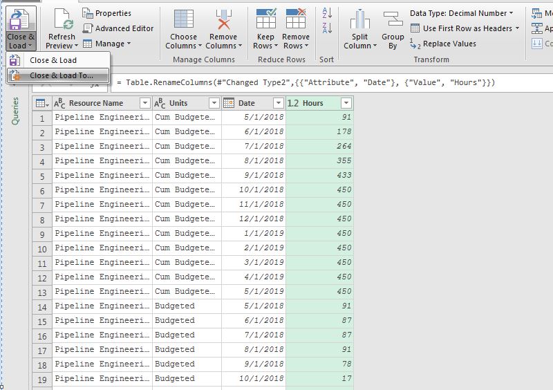
The final step is to rename columns 3 (Attribute) and 4 (Value) to be Date and Hours. You do this by double clicking on the column header and typing the correct text.

Step 16

The query is now finished. The resource name issue has been fixed and the date and hours data are unpivoted. Now you want to return the data to your excel worksheet as a table and use the table to create a Pivot Chart. Click Close and Load To.. in the top left corner of the screen.

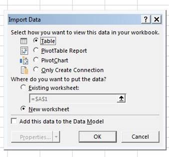
You want the data returned as a table in a new tab so select the following options.